Bringing back the early days of radio, part 1: Background and thinking

I posses a number of very old radio receivers from the beginning of the last century – truly beautiful artefacts from the dawn of wireless communication and I have restored them all to working condition, see below.

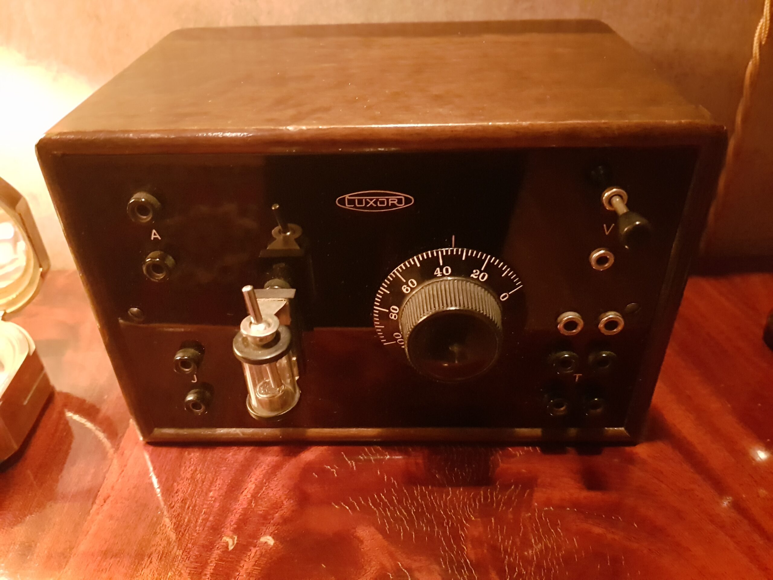
These old receivers were mainly built to receive radio broadcasts on very low frequencies, i.e. Long Wave or LW (roughly 150 – 300 kHz). However, in the part of the world where I live there are no longer any nearby LW transmitters which basically means that I sadly have nothing to listen to.

My way of mitigating this problem is simply to attempt to build a transmitter. I started with acquiring a permit from the national spectrum authority and after a bit of a struggle I received license which allows me to transmit wireless audio anywhere from 148.5 – 283.5 kHz emitting maximum 1 W from the antenna. No turning back now!!!!

First, we need to go through the underlying theory and some math to understand what we need to design and then implement.

To begin, the fundamental objective of radio transmission is to convey information over distance using electromagnetic (EM) waves, although in electronic warfare systems such as jammers the transmitted signal is instead intended to disrupt or deny communication. Conveying information is accomplished through modulation, the process of encoding information (voice, data) onto a carrier wave by altering its properties (amplitude, frequency, phase). Common modulation techniques include Amplitude Modulation (AM), Frequency Modulation (FM) and digital methods like ASK, FSK, PSK, and QAM, using discrete changes in amplitude, frequency, or phase to carry data. Modulation is most commonly achieved by shifting a baseband signal’s frequency range to a new frequency band centered around an RF carrier frequency.

As pointed out, there are a number of different ways to do this but during the early days of wireless communication things were of course simple. Back in the days, the most straightforward way was used which was to use amplitude modulation (AM). AM modulation varies the amplitude of a sinusoidal carrier wave in accordance with the baseband signal, i.e. the audio. This is accomplished by simply multiplying the message signal with the carrier wave in the time domain. To illustrate what happens, the below figure has been generated using Octave. In order to calculate each signal’s frequency spectrum Fourier analysis was used, more precise Discrete Fourier Transform (DFT). Fourier analysis is a family of mathematical techniques, all based on decomposing signals into sinusoids. The Discrete Fourier Transform (DFT) is the family member used with digitised signals.

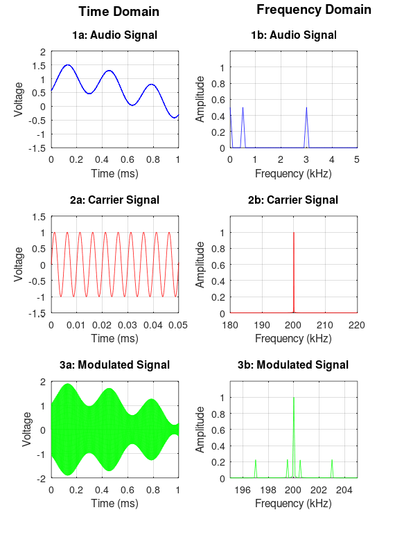
Figure 1a shows a snippet of an audio signal consisting of two superimposed sine tones, one at 500 Hz and one at 3000 Hz, with a 0.5V DC bias. Figure 1b shows that its frequency spectrum is composed of the two frequencies plus a spike for the DC component at 0 Hz. Figures 2a and 2b show the carrier signal, f_c, a pure sinusoid of much higher frequency than the audio signal, 200 kHz. In the time domain, the AM modulated signal consists of multiplying the audio signal by the carrier signal. As shown in 3a, this results in a waveform that has an instantaneous amplitude proportional to the original audio signal. Using wireless lingo, the envelope of the carrier signal is equal to the modulating signal which is the definition af AM. This signal can then be routed to an antenna, converted into a radio wave, and at the other end be detected by a receiving antenna and finally forwarded to an AM receiver which demodulates the signal and outputs the original audio signal again.

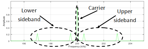
An important property of the Fourier transform is that multiplication in one domain corresponds to convolution in the other domain. Hence, since the time domain signals are multiplied, the corresponding frequency spectrum is a convolution. That is, 3b is found by convolving 1b and 2b. Since the spectrum of the carrier is a shifted Dirac delta function, the spectrum of the modulated signal is equal to the audio spectrum shifted to the frequency of the carrier. This results in a modulated spectrum composed of three components: a carrier, an upper sideband, and a lower sideband, see the figure below.

To understand how the sidebands are generated, the easiest thing to is to derive the governing equation for the AM modulated signal. To begin, using mathematical notation we have the following in our example:

modulation signal (our audio):
$m(t) = A_1 \sin(2 \pi f_1 t) + A_2 \sin(2 \pi f_2 t)$
Note: f₁=500 Hz and f₂=3000 Hz.

carrier signal:
$c(t) = A_c \cos(2 \pi f_c t)$
Note: f_c=200 kHz.

Now, one might wonder why the carrier is there – it does not seem to add anything important and is just a waste of power? This is correct and it is referred to as Double Sideband – Large Carrier (DSB-LC) or “real AM” and was used during the early days of broadcasting (1910s – 1930s). Later on, technology evolved and the carrier was suppressed, a technique called Double Sideband – Suppressed Carrier (DSB-SC) which mitigated the problem where 2/3 of the power was wasted in the carrier at 100% modulation using DSB-LC. However, DSB-LC required less complicated technology, e.g. crystal receivers, and was therefore preferred in the beginning.

The general form for the modulated signal for DSB-LC AM is:

$s(t) = A_c\cos(2 \pi f_c t) \cdot (1 + k \, m(t))$

Note the multiplication operation of two time-dependant functions where the first factor is easily recognised as the carrier signal, c(t). For DSB-SC the “1” in the first factor will disappear and the whole equation will become more intuitive but since we want to go back to the early days of radio broadcasting we need to aim for DSB-LC.

Also note that k is the modulation index which measures the extent of variation in a carrier signal’s amplitude due to the modulating signal, indicating the depth of modulation. For AM the modulation index is simply the ratio of modulating signal amplitude to carrier amplitude, k=A_m/A_c, often expressed in %.

We now substitute the expression for m(t) into s(t) above and we get (I choose not to split the equations although I know it looks bad on a cell phone, please use a large screen for optimal viewing):

$s(t) = A_c \Big( 1 + k \big( A_1 \sin(2 \pi f_1 t) + A_2 \sin(2 \pi f_2 t) \big) \Big) \cos(2 \pi f_c t)$

Expand (again split across lines):
$s(t) = A_c \cos(2 \pi f_c t) + k A_c A_1 \sin(2 \pi f_1 t) \cos(2 \pi f_c t) + k A_c A_2 \sin(2 \pi f_2 t) \cos(2 \pi f_c t)$

Now we remember that:
$\sin x \cdot \cos y=\frac{1}{2}​\Big(\sin(x+y)+\sin(x−y)\Big)$

We use that and then finally arrive at the following expression for the AM modulated signal:

$s(t) = A_c \cos(2 \pi f_c t) + \frac{k A_c A_1}{2} \Big( \sin 2 \pi (f_c+f_1) t + \sin 2 \pi (f_c – f_1) t \Big) + \\ \frac{k A_c A_2}{2} \Big( \sin 2 \pi (f_c + f_2) t + \sin 2 \pi (f_c – f_2) t \Big)$

In the above equation we now clearly see all five spectral components as indicated in figure 3b.

It is now time to design a Long Wave DSB-LC AM transmitter based on the above!

Please have a look in part 2: Design.